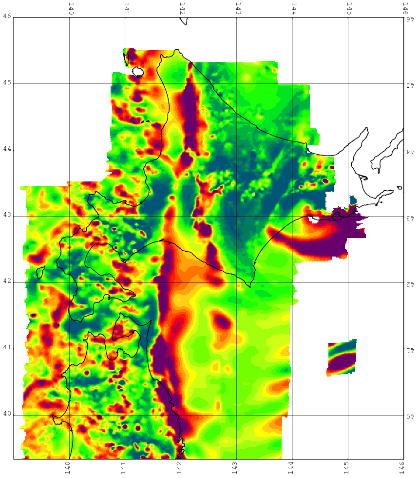
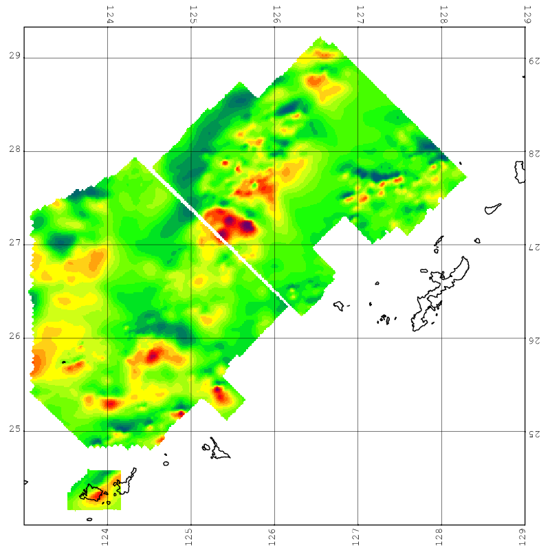
 To show the general view of the data in this report, color-graded
magnetic anomaly maps were produced from the data for five districts,
as seen below.
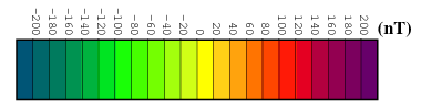
Here a common color-scale grading is used as is shown on the right.
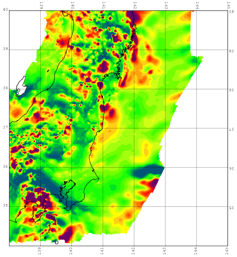
To show the general view of the data in this report, color-graded
magnetic anomaly maps were produced from the data for five districts,
as seen below.
Here a common color-scale grading is used as is shown on the right.
| GSJ Open-file Report, no. 516 | November, 2009 |
In 2005, the Geological Survey of Japan, AIST (GSJ)
published the "Aeromagnetic Database of Japan" (GSJ, 2005) as a
compilation of existing data of aeromagnetic surveys accumulated at GSJ.
This publication includes two database components, "survey database"
and "anomaly database", and covers almost all available aeromagnetic
data of reconnaissance surveys over the Japanese Islands.
As the database was compiled so as to reserve the
characteristics (accuracy, resolving power, etc. coming from the survey
specification) of surveys, it contains the data quite near to raw
observation.
It is natural that each dataset in the "Aeromagnetic Survey Database of
Japan" (Nakatsuka et al., 2005) reflects directly the survey specification
of each survey.
Also the "Aeromagnetic Anomalies Database of Japan" (Nakatsuka and Okuma,
2005) is built without applying any sophisticated technique of data
processing.
In this report, a data reduction technique using the
equivalent source analysis was applied to the data above in order to
derive a magnetic anomaly map for imaging subsurface structure with
nearly equal quality all over Japan.
The magnetic anomaly distribution at a smooth surface of 1,500 meters
above terrain was compiled at the grid size of 0.1 minute of latitude
and longitude.
The aeromagnetic data accumulated at GSJ and the data of
NEDO Curie Point Surveys, i.e., all data included in the "Aeromagnetic
Anomalies Database of Japan" (Nakatsuka and Okuma, 2005), were utilized
to this time compilation of the quality-equalized magnetic anomaly map.
Table-1 is the list of surveys contributed to this compilation.
In order to generate altitude data of the smooth reference
surface of 1,500 meters above terrain (on which the magnetic anomalies are
reduced), we used the data of Digital Maps "50m DEM" (Japan-I, Japan-II,
Japan-III) published by the Geographical Survey Institute, MLIT, Japan.
| Name | Year of survey | GSJ Map Publication #, Area-name [Year] | Data Source Organization |
|---|---|---|---|
| NEDO_KSH | 1981 | ** (NEDO: Kyushu) | NEDO |
| NEDO_THK | 1981-82 | ** (NEDO: Tohoku) | NEDO |
| NEDO_HKD | 1982 | ** (NEDO: Hokkaido) | NEDO |
| NEDO_CHB | 1982 | ** (NEDO: Chubu) | NEDO |
| NEDO_KNT | 1982 | ** (NEDO: SouthTohoku-Kanto-Tokai) | NEDO |
| NEDO_CGK | 1983 | ** (NEDO: Chugoku-Shikoku) | NEDO |
| SADO_N | 1968 | 1.-2 Murakami-Yahiko [1972] | GSJ |
| NOSHIRO | 1968 | 22. NishiTsugaru-Sakata (portion) [1978] | GSJ |
| ISHIKARI | 1969 | 2.-4 Rumoi-Sapporo [1972] | GSJ |
| SADO_S | 1969 | 1.-3 Yahiko-Itoigawa [1972] | GSJ |
| SAKATA | 1969 | 1.-1 Sakata-Murakami [1972] | GSJ |
| RISHIRI | 1970 | 2.-2,3 Rishiri-Rumoi [1972] | GSJ |
| ABUKUMA | 1970 | 6. Kesennuma-Hitachi [1974] | GSJ |
| SOYA | 1971 | 3. Soya-Abashiri [1973] | GSJ |
| AMAKUSA | 1971 | 5. Nagasaki-Sendai [1973] | GSJ |
| HITACHI | 1971 | 7. Hitachi-Kamogawa [1974] | GSJ |
| TOKAI | 1972 | 4. Omaezaki-Toyohashi [1973] | GSJ |
| DOTO | 1972 | 8. Atsukeshi-Erimo [1974] | GSJ |
| DONAN | 1972 | 9. Hakodate-Erimo [1974] | GSJ |
| MIYAZAKI | 1973 | 16. Nobeoka-Satamisaki [1977] | GSJ |
| OKUJIRI | 1973 | 10. Shakotan-Okujiri [1974] | GSJ |
| HOKURIKU | 1973 | 11. Wajima-Fukui [1975] | GSJ |
| SHMOKITA | 1973 | 12. Shiriyazaki-Kesennuma [1975] | GSJ |
| TOTTORI | 1974 | 13. Fukui-Oki [1977] | GSJ |
| KUMANO | 1974 | 14. Toyohashi-Kushimoto [1977] | GSJ |
| TEMPOKU | 1974 | 17. Tempoku [1977] | GSJ |
| KAMUIKTN | 1974 | (Kamuikotan) [ms.] | GSJ |
| MUROTO | 1975 | 15. Kushimoto-Nobeoka (1-3) [1977] | GSJ |
| TOKACHI | 1975 | 18. Tokachi [1977] | GSJ |
| ASHIZURI | 1975 | 15. Kushimoto-Nobeoka (3,4) [1977] | GSJ |
| HIDAKA | 1976 | 19. Hidaka [1978] | GSJ |
| TSUGARU | 1976 | 21. Okujiri-Tsugaru [1978] | GSJ |
| GOTO | 1977 | 23. Goto-Koshikijima [1978] | GSJ |
| DAISETSU | 1977 | 20. Daisetsu [1978] | GSJ |
| AKITA | 1977 | 22. NishiTsugaru-Sakata [1974] | GSJ |
| TANE | 1977 | 25. OsumiPen.-Tanegashima [1980] | GSJ |
| KITAMI_A | 1978 | 24. Kitami (1.Abashiri) [1979] | GSJ |
| KITAMI_M | 1978 | 24. Kitami (2.Mombetsu) [1979] | GSJ |
| TOYAMA | 1978 | 26. Sado-NotoPen. [1980] | GSJ |
| BOSO | 1978 | 27. Boso-Izu [1980] | GSJ |
| JOBAN1 | 1980 | 28. Joban (1,2) [1981] | GSJ |
| JOBAN2 | 1980 | 28. Joban (3,4) [1981] | GSJ |
| SANRIKU1 | 1980 | 30. Sanriku (3,4) [1982] | GSJ |
| SANRIKU2 | 1980 | 30. Sanriku (1,2) [1982] | GSJ |
| ERIMOSMT | 1980 | (ErimoSeamount) [ms.] | GSJ |
| KANTO1 | 1981 | 31. Kanto (1,2) [1982] | GSJ |
| KANTO2 | 1981 | 31. Kanto (3,4) [1982] | GSJ |
| SURUGA | 1977-78 | * (JICA) SurugaBay [1979] | JICA, GSJ |
| URAGA | 1980-81 | * (JICA) UragaStrait [1983] | JICA, GSJ |
| ISEWAN | 1982-85 | * (JICA) IseBay [1986] | JICA, GSJ |
| OKINAWA1 | 1982-83 | 32. NW of OkinawaJima [1984] | GSJ |
| OKINAWA2 | 1983-84 | 33. W of OkinawaJima [1985] | GSJ |
| MIYAKO | 1985-87 | 34. N of MiyakoJima [1989] | GSJ |
| ISHIGAKI | 1986-89 | 35. SenkakuIs. [1993] | GSJ |
| OSHIMA | 1978,86 | 36. IzuOshima [1994] | GSJ, NAS |
| ITO | 1989 | 37. ItoCity [1994] | GSJ |
| UNZEN | 1991 | 38. Unzen [1994] | NAS, GSJ |
| IRIOMOTE | 1992 | 39. IriomoteJima [1994] | GSJ |
|
NEDO : New Energy Development Organization,
GSJ : Geological Survey of Japan, JICA : Japan International Cooperation Agency, NAS : Nakanihon Air Service Co. Ltd. ** (NEDO: xxxx) : magnetic maps before compilation are not published. * (JICA) : published by JICA. | |||
First, as a reference altitude surface to which magnetic
anomalies are to be reduced, the altitude data of a smooth surface of
1,500 meters above terrain were generated from the 50m DEM (digital
elevation model) data (Digital Maps by the Geographical Survey Institute,
MLIT, Japan).
Next, the aeromagnetic survey data of each survey were
converted into the form of numbers of point observations, as if they
are the distribution of random observations apparently.
Then the altitude reduction procedures (Nakatsuka, 2007) in use of
equivalent source technique as developed by Nakatsuka and Okuma (2006)
were applied to those observational data to acquire the magnetic anomaly
distribution on the reference surface.
Actual process of calculations was performed under UTM coordinate
systems.
To save resultant magnetic anomaly distribution in a form
independent to the map projection, the grid-interpolation into
latitude-longitude system was applied and the data were divided into
areas of the primary mesh (40 minutes latitude × 1 degree longitude).
Then the final data of each primary mesh area were composed of mesh
values (magnetic anomaly values and reference altitude values) at the
mesh points of every 0.1 minute intervals in latitudes and longitudes.
With respect to the more detailed explanation of processing
and process parameters, refer to the Japanese description.
This report consists of the files listed in Table-2.
Among them, "allmgc.tgz" is a 'gzip' compressed 'tar' archive with a size
of about 97MB, and it contains all data files of magnetic anomalies.
If all those data files are uncompressed and extracted from the archive,
207 files with the size of 800MB in total will be recovered.
Their filenames are listed in the file "allmgclist.html".
| Filename | Contents |
|---|---|
| 0516index.html | Cover page HTML (in Japanese) |
| index.html | Table of contents |
| japanese.html | Description HTML in Japanese |
| english.html | Description HTML in English |
| allmgc.tgz | Gzip compressed tar archive of 207 data files [97 MB] |
| allmgclist.html | List (HTML) of 207 data files in 'allmgc.tgz' archive |
| cm141N.png | Magnetic anomaly maps of 5 districts |
| cm141.png | |
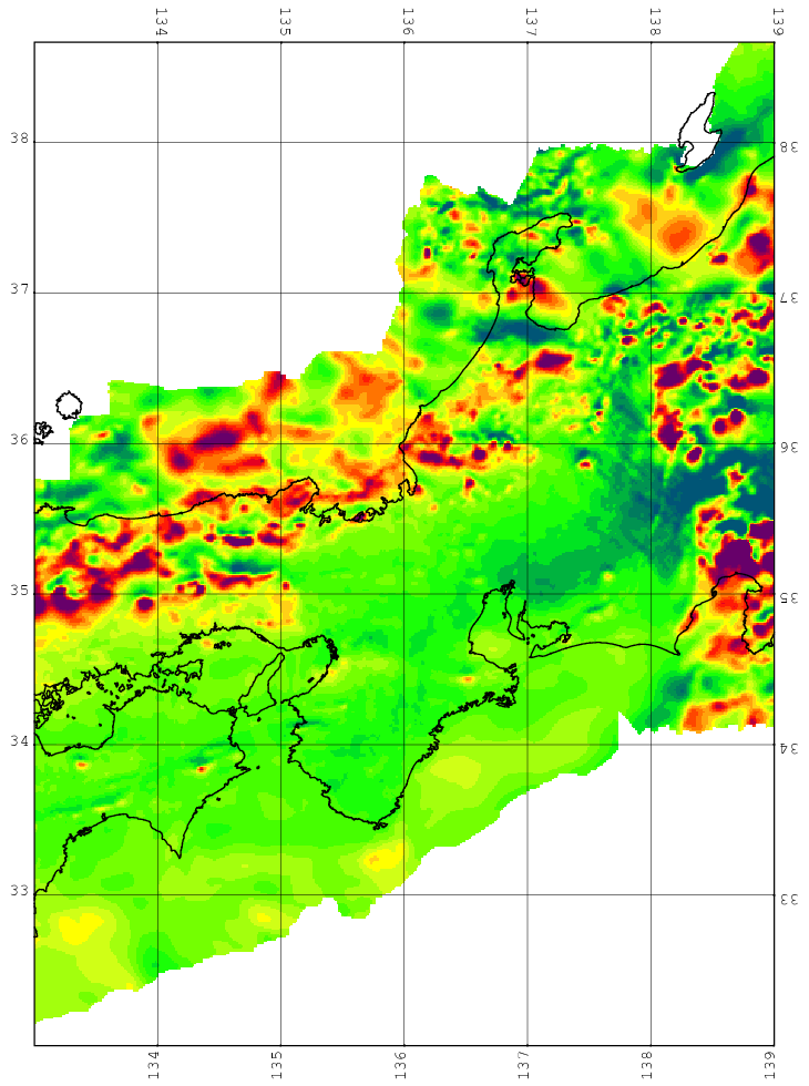
| cm135.png | |
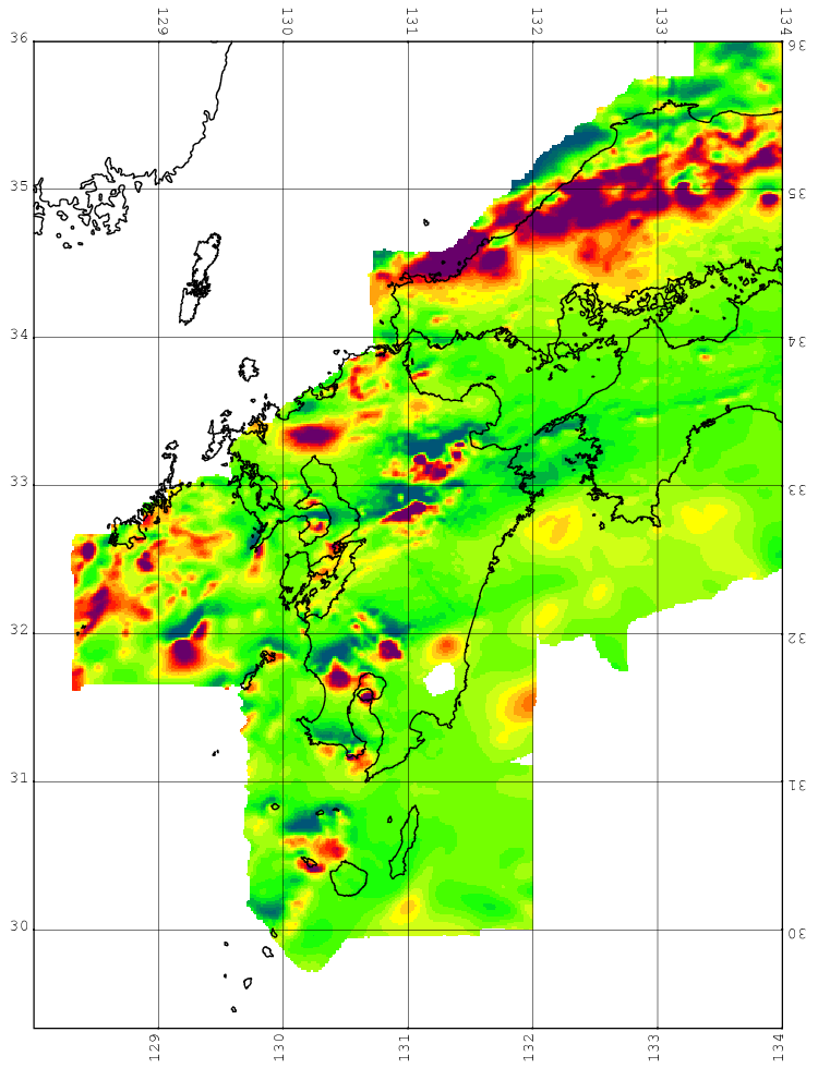
| cm129.png | |
| cm123.png | |
| legend.png | Color grading legend |
| Line | Contents | |
|---|---|---|
| 1 | Comment | |
| 2 | Header-1 | |
| 3 | Header-2 | |
| 4–24644 | Magnetic values grid data | 401×601 values |
| 24645 | Header-1 | |
| 24646 | Header-2 | |
| 24647–49287 | Altitude values grid data | 401×601 values |
name |
offset |
cols |
format | Contents |
|---|---|---|---|---|
| (Comment line) | ||||
| 0 | 4 | A4 | "## " | |
zone | 4 | 8 | A8 | "cm123 ", "cm129 ",
"cm135 ", "cm141 ", or "cm141N "
|
| (Header-1) | ||||
area | 0 | 8 | A8 | 4 digit mesh code + space (4 columns) |
nc | 8 | 4 | I4 | 399 (projection ID number) |
- | 12 | 4 | 4X | (space) |
iorg | 16 | 8 | I8 | Origin information of the projection,
ispa = ispb = 0.iorg and korg are the origin latitude and
longitude in minutes, respectively.(Actually, iorg = 0 .) |
korg | 24 | 8 | I8 | |
ispa | 32 | 8 | I8 | |
ispb | 40 | 8 | I8 | |
| (Header-2) | ||||
ixs | 0 | 12 | I12 | Coordinate values (in 0.001 minutes) to N
(ixs) and to E (iys) of the Southwest corner.
Given as values relative to the Origin defined above. |
iys | 12 | 12 | I12 | |
mszx | 24 | 6 | I6 | Grid intervals (in 0.001 minutes) to N
(mszx) and to E (mszy).(Actually, mszx = mszy = 100 .) |
mszy | 30 | 6 | I6 | |
mx | 36 | 6 | I6 | Numbers of grids to N (mx) and to E
(my) counting both ends.(Actually, mx = 401, my = 601 .) |
my | 42 | 6 | I6 | |
vnul | 48 | 8 | F8.1 | Special value to indicate lack of valid data (actually, 9999.9). |
To show the general view of the data in this report, color-graded
magnetic anomaly maps were produced from the data for five districts,
as seen below.
Here a common color-scale grading is used as is shown on the right.